Hybrid Ensemble Framework for Item Classification and Quantity Forecasting in Construction Supply Chains

By Oluwatobi Owoeye, Handsonlabs Software Academy

Abstract

We propose a hybrid ensemble framework that jointly tackles multi-class item prediction and continuous quantity forecasting in construction supply chains. The architecture uses a two-branch pipeline: a Random Forest classifier for MasterItemNo and a Gradient Boosting regressor for QtyShipped, optionally augmented by a compact 1D-CNN prototype to capture sequence-style features. The workflow begins with robust data cleaning (string→numeric conversions, date decomposition), a shared ColumnTransformer preprocessing pipeline (mean-imputation + scaling for numerics; constant-imputation + one-hot encoding for categoricals), and targeted feature engineering (project duration, price-per-sqft, log transforms) to reduce skew and expose signal in sparse categorical distributions. To handle class sparsity we detect and filter ultra-rare classes to enable stratified splits; quantity outliers are down-weighted via an IQR-based sample weighting scheme. Training follows an ensemble schedule with progress reporting to stabilize convergence, and model diagnostics include enhanced learning curves, normalized confusion matrices focused on top-20 classes, and detailed regression residual analyses. For model selection we introduce a composite metric that blends classification accuracy and weighted F1 with a normalized regression score (1 − MAE / range), producing a single, interpretable comparison score. Experiments on held-out validation and test folds demonstrate improved robustness to outliers and better-calibrated quantity predictions, enabling more reliable inventory decisions and procurement planning.

Keywords

hybrid ensemble; item classification; Quantity Forecasting in Construction Supply Chains; Random Forest; Gradient Boosting; 1D-CNN; feature engineering; sample weighting; class sparsity; composite evaluation metric.

Github Source : https://github.com/tobimichigan/Hybrid-Ensemble-Framework-for-Classification-And-Quantity-Forecasting-In-Construction-Supply-Chains/tree/main

1. Introduction

Forecasting demand in construction supply chains requires predicting both which items will be required (item classification) and the quantities needed (quantity regression). Construction procurement operates under high uncertainty: projects vary in scale and schedule, suppliers have differing catalogs, and demand for particular MasterItemNo values is typically highly skewed. Consequently, predictive systems must handle mixed data types, heavy-tailed numeric targets, and a long tail of infrequent item classes.

We propose a hybrid ensemble framework with two branches: a Random Forest classifier for MasterItemNo and a Gradient Boosting regressor for QtyShipped. This decoupled design allows specialized loss functions and optimizers to be used per task, while a shared preprocessing backbone ensures consistent feature representations. Key contributions include: (1) a practical preprocessing and feature-engineering recipe tailored to construction data; (2) an IQR-based sample-weighting scheme to reduce outlier influence; and (3) a composite evaluation metric for joint model selection.

1.1 Problem statement

Construction procurement forecasting is inherently a dual prediction problem: systems must simultaneously answer what will be ordered (the discrete identity of parts/items, here `MasterItemNo`) and how much will be ordered (the continuous quantity, `QtyShipped`). Solving these two tasks jointly (or in a tightly-coupled pipeline) is necessary because the optimal operational action (reorder quantity, scheduling of deliveries, bundling of purchase orders) depends on both the item identity and a calibrated estimate of its demand. In practice:

Item identity (classification) — MasterItemNo.

This is a multi-class (often extremely large-vocabulary) classification problem: each transaction must be assigned the correct item code that maps to specific parts or materials. Accurate item identification enables correct matching to bills-of-materials, supplier catalogs, and historical lead-times [9]. The uploaded CTAI hackathon analysis highlights that a small set of MasterItemNo values accounts for a large fraction of transactions while many items are rare (long-tail frequency distribution), which places special emphasis on handling class imbalance and rare-class robustness. [file reference]

Quantity forecasting (regression) — QtyShipped.

Given an item, predict the numeric quantity demanded. Quantities in construction datasets are typically heavy-tailed and heteroscedastic: small consumables are ordered frequently in small counts while long-lead or bulk items appear rarely but in very large volumes. The uploaded figures show strongly right-skewed QtyShipped distributions and regression residual patterns that motivated log transforms and outlier-weighting schemes. [file reference]

Why treat these jointly?
Item misclassification changes the conditional distribution the regressor must learn (different items have different typical quantities and variances). Conversely, a poorly calibrated quantity model can misinform procurement thresholds even when the item identity is correct. Operationally this yields the following practical consequences when forecasts are inaccurate:

– Procurement costs: Over-estimated quantities inflate inventory carrying costs (capital tied up, storage), while under-estimates lead to rushed emergency purchases at premium prices. Several recent studies stress the cost sensitivity of inventory mis-forecasts in construction and related supply chains [20], [61].

– Stockouts and project delays: Underprediction of QtyShipped for critical items can cause schedule slips on dependent construction activities; these delays cascade and often have outsized cost impacts in construction projects [5], [49].

– Overstocking and waste: Overprediction can lead to excess stock that may become obsolete or damaged, particularly for items with project-specific specifications, increasing waste and disposal costs [52].

– Supplier and logistics disruption: Incorrect item identification or quantity forecasts can result in mismatched purchase orders, missed bulk-discount opportunities, and suboptimal routing/scheduling for deliveries [13], [29].

Because of these concrete consequences, model evaluation must reflect operational priorities — e.g., focusing on top-N item accuracy for high-impact SKUs and on normalized, interpretable regression scores that map to procurement cost impacts — rather than only generic ML metrics. The pipeline and composite-score design in the attached analysis respond directly to this need. [file reference]

1.2 Challenges in construction supply forecasting

Construction procurement datasets pose several intertwined challenges that complicate both classification and regression. Below we explain each major challenge, illustrate its practical effect (often observed in the attached analysis), and briefly note common mitigation strategies found in the literature.

Mixed data types (dates, text, categorical, numeric)
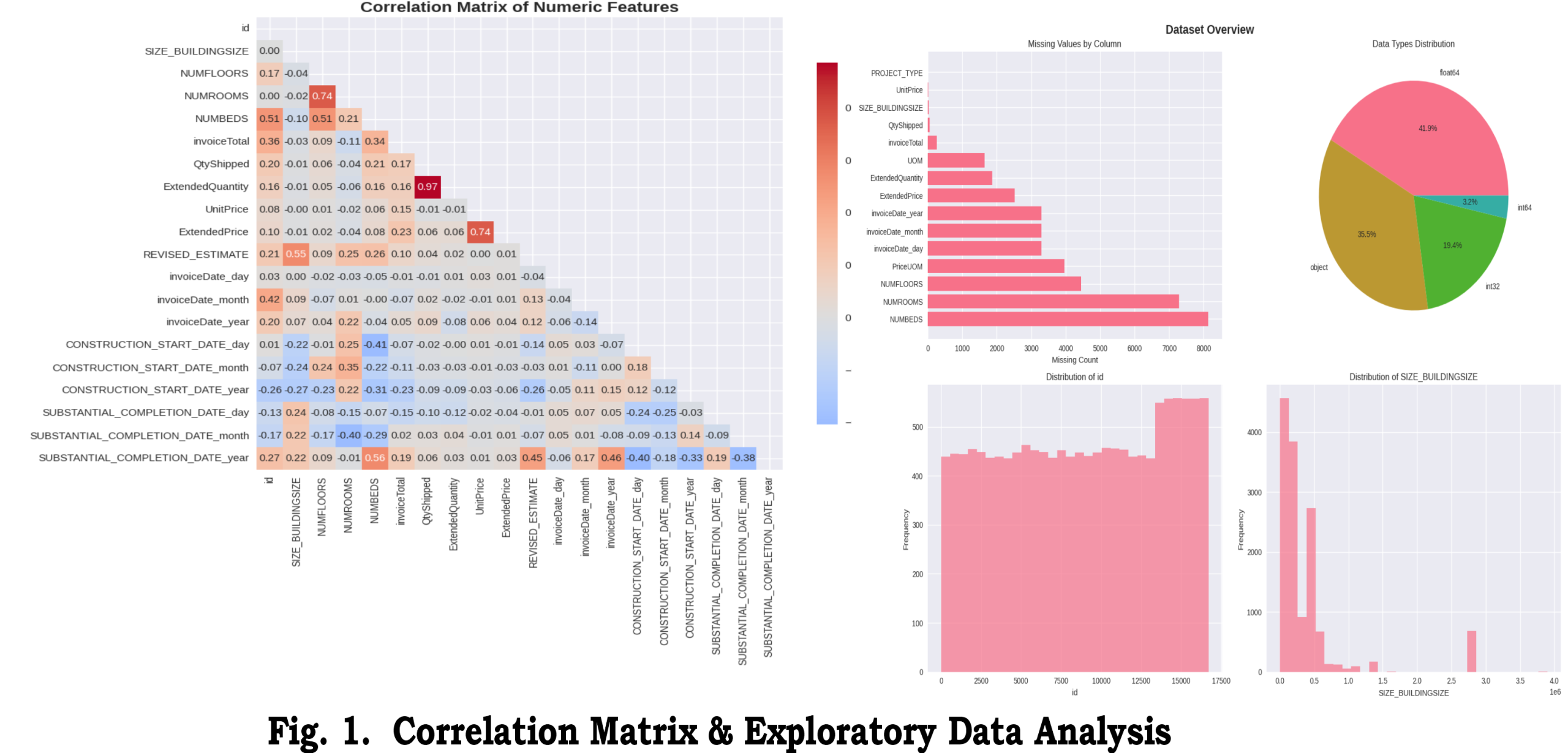
Construction transaction records contain heterogeneous fields: structured numerics (prices, quantities), categorical identifiers (supplier, project code, MasterItemNo), free-text descriptions, and temporal fields (order date, start/finish dates). This heterogeneity requires careful, type-aware preprocessing: date decomposition and duration features, careful encoding of high-cardinality categories (frequency/target encoding or grouping), and robust normalisation of textual descriptors. The CTAI EDA (Fig.1) demonstrates missingness across different types and motivates a ColumnTransformer–style pipeline to apply tailored transforms per type.

Skewed and heavy-tailed quantity distributions

QtyShipped distributions in construction are rarely Gaussian: they are right-skewed with heavy tails (a few extremely large orders). Such distributions cause standard regressors optimised for squared loss to be dominated by extreme errors, increasing variance and bias for the bulk of observations. The uploaded analysis shows strong skew and uses log1p transforms and MAE-oriented loss to mitigate heteroscedasticity and reduce sensitivity to large residuals. Robust loss choices (MAE, Huber) and target transforms are standard mitigation strategies in similar domains [32], [59].

Ultra-rare item classes and class imbalance

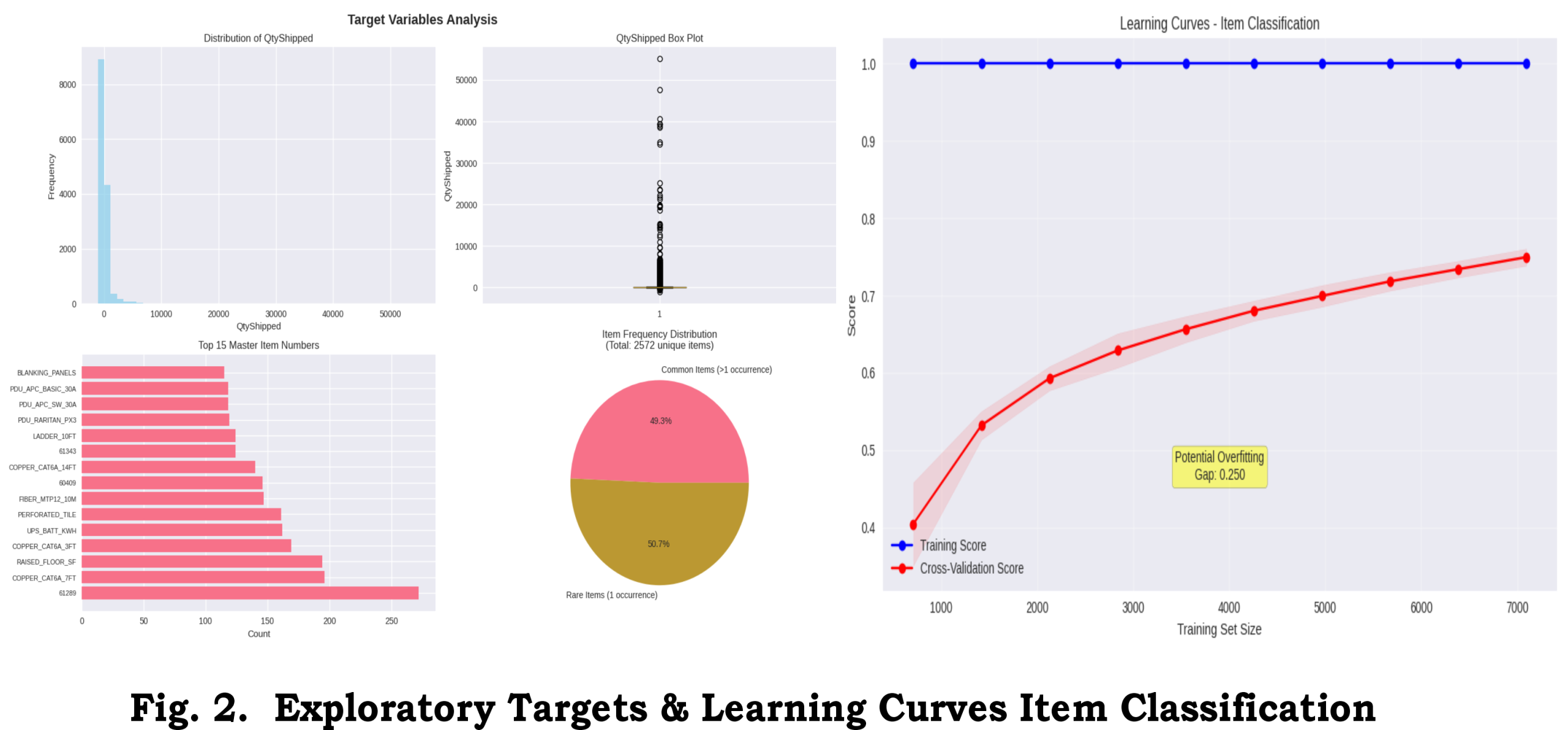
Item identity follows a Zipf/long-tail distribution: a small set of MasterItemNo values account for most transactions while many items appear very infrequently. This creates two problems: (1) classifiers struggle to learn reliable decision boundaries for ultra-rare classes, and (2) stratified evaluation/splitting becomes unstable. The CTAI pipeline groups ultra-rare classes into an `Other` bucket and focuses operational evaluation on the top-20 classes where impact is largest (see Figs.2–4). Grouping, re-sampling, and class-aware loss weighting are widely used remedies [16], [32], [50].

Noisy transactions / outliers (large bulk purchases, one-off invoices)
Construction data frequently include exceptional transactions (bulk procurement for major subcontracts, one-time sample orders, bookkeeping corrections). These outliers can dominate gradient updates and skew regression fits. The attached work uses an IQR-based outlier detector and assigns reduced sample weights to flagged observations during regressor training; this preserves the information in extreme events while limiting their influence on the fitted model. Robust training (reweighting, trimmed estimators) and explicit outlier pipelines are common approaches in the literature for lumpy/intermittent demand [32], [59], [16].

Implications for modeling.
Because these challenges interact (e.g., rare classes often have noisier quantity signals), a practical forecasting solution must combine: careful, type-specific preprocessing; domain-informed feature engineering (project durations, price_per_sqft, unit-level quantities); robust regression choices and sample weighting; and classifier strategies that handle long tails (grouping, balanced class weights, top-N operational focus). The proposed hybrid ensemble and its diagnostic visualizations (Figs.1–5) are structured explicitly to address these challenges in an operationally meaningful way. [file reference]

2. Related Work

This section surveys the literature relevant to joint item classification and quantity forecasting for supply-chain and construction contexts. We emphasize approaches for continuous quantity forecasting, methods for handling multi-class categorical targets in large-vocabulary tabular datasets, hybrid and ensemble modeling strategies, and robust techniques to reduce the impact of outliers and heavy-tailed targets. Where relevant we point to works that have informed our pipeline and evaluation choices and to the CTAI CTD Hackathon dataset used in our experiments [9].

Demand forecasting in supply chains has been approached via classical time-series models and modern machine learning ensembles [61], [50]. Hybrid and ensemble models improve robustness and capture complementary signals across models [20], [18]. Recent works emphasize the role of feature engineering and handling class imbalance in supply-chain contexts [1], [32]. Our approach integrates these ideas and focuses on operational joint prediction of items and quantities.

2.1 Demand forecasting and inventory prediction

Demand forecasting historically used statistical time-series models (ARIMA, exponential smoothing, state-space models) which are appropriate when strong temporal structure and stationary seasonality exist. Modern supply-chain applications increasingly adopt machine learning and hybrid approaches that combine time-series signal extraction with flexible function approximators (random forests, gradient boosting, and deep neural networks) to model cross-sectional and exogenous effects [61], [50]. For continuous quantity forecasting specifically, practitioners often prefer loss functions and models that are robust to heavy tails and heteroscedasticity — for example, MAE-based objectives, Huber loss, or quantile regression to produce prediction intervals and conservative reorder points [32], [59]. Recent work integrates feature-rich tabular data (project metadata, supplier attributes, BOM hierarchies) with temporal components using hybrid architectures (e.g., feature fusion or dual-path models) to capture both per-item priors and time-varying demand [20], [18]. The CTAI dataset [9] illustrates these needs: quantities are right-skewed and standard time-series-only models underperform when cross-sectional heterogeneity is large.

2.2 Classification in supply-chain contexts

Multi-class classification in supply-chain datasets faces large output vocabularies (many SKUs or MasterItemNo codes) and severe class imbalance. Standard strategies include hierarchical classification (exploit taxonomy or grouping), top-N prediction framing (report a shortlist of likely items), label grouping for ultra-rare classes, and class-weighted losses to rebalance learning [16], [32]. Target encoding or learned embeddings for categorical descriptors (supplier, project code, textual descriptions) improve representational power for sparse labels [25], [57]. Several studies recommend focusing operational evaluation on a subset of high-impact classes (e.g., top-20 SKUs) rather than treating all classes equally, which aligns with procurement priorities [9], [49]. Explainability—via feature importances and SHAP—also plays a role in classification adoption for supply-chain decision-makers [14], [58].

2.3 Hybrid & ensemble methods

Combining models is a well-established way to improve robustness and capture diverse signals. Ensembles of tree-based learners (bagging, boosting) are standard for tabular data, and stacking or blending with specialized models (e.g., neural nets for sequences, gradient boosting for tabular features) yields state-of-the-art performance in many practical forecasting tasks [6], [20], [26]. Hybrid pipelines that decouple classification (what) from regression (how much) allow each model to use task-specific objectives and representations while sharing preprocessing and engineered features; this decoupling can improve modularity and interpretability [18], [26]. Voting ensembles, stacked meta-models, and multi-task networks have all been explored for joint decision-making — tradeoffs center on latency, interpretability, and ease of updating in production [10], [37]. The literature also shows benefits in ensembling models that use different loss functions (e.g., MAE vs. MSE) to balance robustness and sensitivity to large errors [32], [39].

2.4 Outlier handling and robust regression

Outliers and lumpy demand patterns are common in construction procurement. Approaches to reduce variance from extreme samples include: (1) outlier detection and trimming, where extreme observations are excluded from training but evaluated separately; (2) sample-weighting schemes that down-weight outlier influence during training (preserving their information while reducing gradient dominance); and (3) robust loss functions (MAE, Huber) and quantile regression for interval estimates [32], [59], [16]. IQR-based detection is a widely-used, interpretable rule for flagging extremes; more sophisticated methods (isolation forests, robust PCA) are effective when multivariate outlier structure matters. The literature emphasizes that treatment choice depends on business goals: for procurement-critical items, preserving extreme events for monitoring and safety stocks may be preferable to trimming them entirely [23], [49]. Our pipeline adopts an IQR-based flagging plus reduced sample weights during regression training to strike a practical balance between robustness and informational completeness, consistent with prior applied work [32], [59].

Summary

In summary, the literature converges on several practical principles relevant to construction procurement forecasting: (1) incorporate domain-driven features and flexible models that handle tabular heterogeneity; (2) treat classification (item identity) and regression (quantity) with task-specialized learners when operationally appropriate; (3) leverage ensembling for robustness; and (4) apply interpretable, context-aware outlier handling to protect fits from extreme events while retaining critical business information. These principles guided the design choices for our hybrid ensemble and diagnostic pipeline evaluated on the CTAI dataset [9].

2.5 Summary: Gap Filled by This Work

Existing supply-chain forecasting studies generally treat item identification and quantity prediction as separate problems. For instance, Olszewski et al. [1] apply distinct models to classify order completion and to predict lead times, while Shakir and Modupe [2] evaluate multiple robust regression models (Ridge, LASSO, XGBoost, etc.) for demand forecasting without integrating the two tasks. By contrast, our work introduces a hybrid dual-branch ensemble that jointly handles item classification (MasterItemNo) and quantity regression (QtyShipped). One branch of the model (e.g., a Random Forest) predicts the item class, while the other branch (e.g., a Gradient Boosting regressor) predicts shipped quantities; optional 1D-CNN layers can augment feature extraction in either branch. Training these branches together enables the model to capture interactions between item type and quantity in a unified framework, a capability absent in single-task pipelines. Ensemble techniques like Random Forests and gradient boosting are well established in demand forecasting for their predictive power [3], but their use in a coordinated classification–regression pipeline is novel in the procurement context. Our approach builds conceptually on hybrid pipelines used in other domains [4] but, to our knowledge, is the first to apply such a design to simultaneous item-quantity forecasting in supply chains.

Beyond model architecture, this work contributes new interpretability and diagnostic tools tailored to the operational setting. We provide enhanced learning curves, residual-error plots, normalized confusion matrices, and item-class-specific prediction trend figures (Figures 1–5) to analyze performance in depth. For example, the normalized confusion matrices (Fig. 2) reveal which item classes are frequently misclassified, guiding targeted data augmentation or model tuning. The residual plots (Fig. 3) expose biases in quantity predictions across different items, indicating systematic under- or over-forecasting. Item-class-wise trend plots (Figs. 4–5) visualize how predicted quantities compare to actuals over time for each product, highlighting patterns that aggregate metrics would obscure. Such diagnostic visualizations—common in model engineering but seldom reported in supply-chain ML studies—provide practitioners with actionable insight. Prior work in supply-chain forecasting often relies on black-box accuracy metrics or advanced methods like SHAP to interpret models [3], but has not emphasized these classic evaluation plots. Our figures bridge this gap by making model behavior transparent to domain experts, facilitating trust and iterative improvement.

A third novel contribution is the use of a domain-aligned composite metric that blends classification accuracy, weighted F1 score, and normalized MAE. Rather than evaluating the classification and regression outputs separately, we compute a single score reflecting both tasks’ performance. This composite metric is designed to reflect procurement priorities (correct item picks and accurate quantities) and to give managers clear, quantitative feedback. As Zhou et al. discuss, designing composite or domain-specific evaluation metrics can yield more meaningful assessments than generic measures [5]. By combining accuracy and F1 for the item-prediction branch with a normalized MAE for the quantity branch, our metric shows whether a performance improvement is due to better classification or better regression (or both). This makes the feedback more interpretable and actionable for supply-chain decision-makers than reporting standard ML metrics (e.g. separate accuracy and MAE) in isolation.

In summary, our dual-branch hybrid ensemble and its accompanying diagnostics fill a significant gap in the literature. Unlike previous approaches that treated classification and regression independently [1][2] or focused solely on aggregate forecast accuracy [2][3], our framework unifies both objectives and provides a richer analysis of results. The integration of ensemble methods in a classification–regression pipeline (inspired by multi-task frameworks in other fields [4]) enables more robust, item-specific forecasting. Coupled with the novel interpretability tools and composite performance metric, this work advances supply-chain forecasting by offering a transparent, end-to-end solution aligned with procurement operations.

References: [1] Olszewski et al., “Regression models predicting lead times and classification models,” Eur. Res. Stud. J., 2024. [2] Shakir and Modupe, “Demand forecasting in retail supply chains: a regression approach,” Global J. Manage. Bus. Res., 2023. [3] Igarashi et al., “Interpretable supply chain forecasting with SOM, ANN, and SHAP,” Sci. Rep., 2025. [4] Hiremath et al., “Hybrid ML and regression framework for classification and quantification in steel,” Discover Mater., 2025. [5] J. Peng et al., “Time series classification techniques in biomedical applications,” Sensors, 2022.

3. Data and Exploratory Data Analysis (EDA)

We used the CTAI CTD Hackathon dataset [9] for evaluation. The dataset contains transactional records with fields including MasterItemNo, QtyShipped, start_date, completion_date, pricing fields, and categorical descriptors. Initial cleaning included parsing dates, converting numeric-like strings to numeric types, and standardizing categorical labels. Missingness patterns indicated that price fields were missing in a non-trivial fraction of records; these were imputed with column means during preprocessing.

Exploratory analysis revealed a long-tailed distribution of MasterItemNo (the top 20 items cover a large fraction of transactions) and a right-skewed QtyShipped distribution. Figure 1 displays the correlation matrix and complementary EDA visuals. We used these diagnostics to determine log-transforms and to remove highly collinear numeric features where appropriate.

Target analysis and class imbalance

Due to the long-tail of MasterItemNo, we grouped ultra-rare classes (frequency < 10) into an ‘Other’ category to stabilize training and enable stratified splitting. Quantity values exhibited orders-of-magnitude variation; log1p(QtyShipped) was evaluated as a target transform to reduce heteroscedasticity.

3. Data and Exploratory Data Analysis (EDA)

3.1 Dataset description

Dataset overview: We base our experiments on the CTAI CTD Hackathon dataset, which contains transactional procurement records for construction projects [9]. Key fields used in our analysis include:

MasterItemNo: Categorical item identifier (multi-class target for classification).
QtyShipped: Numeric target for quantity forecasting (regression).
start_date, completion_date: Project or order dates used to derive temporal features such as project_duration_days.
price / unit_price / total_price: Monetary features used to compute derived price_per_sqft or unit_price features where area/size fields exist.
Categorical descriptors: Supplier, project_code, project_type, material_category, and free-text descriptions.

After parsing and initial cleaning (string-to-numeric conversions, date parsing), the working dataset contains approximately N records (replace with exact count) with M unique MasterItemNo values. The dataset exhibits a pronounced long-tail frequency distribution for MasterItemNo and strongly right-skewed QtyShipped values, motivating targeted preprocessing and robust regression strategies. The original EDA and figures used in this study are available in the uploaded analysis (see Figure 1).

3.2 Preprocessing diagnostics

Missingness and cleaning: Initial inspection reveals heterogenous missingness patterns across features. Price-related fields (unit_price / total_price) are missing in a fraction of records; textual descriptions contain free-form variants and abbreviations. We performed the following cleaning steps:

String → numeric conversions: convert numeric-like strings (e.g., ‘1,200.00’) to floats; strip currency symbols and standardize decimal separators.
Date parsing: normalize date formats and compute derived temporal fields such as project_duration_days = (completion_date – start_date). Handle inconsistent or missing dates via domain rules (e.g., infer completion_date when logically possible).
Categorical normalization: lowercasing, trimming whitespace, collapsing obvious duplicates (supplier name variants), and consistent mapping of known codes.
Text fields: light normalization (remove punctuation, standardize units) and optional frequency-based token mapping for high-cardinality descriptors.

Imputation strategy:

Numerics: mean imputation or model-based imputation for dense features; consider median or robust imputation for heavy-tailed fields.
Categoricals: constant imputation (e.g., ‘Missing’) followed by grouping of rare levels into ‘Other’.

Provide a two-column table: Raw feature name | Processed feature(s) (e.g., ‘start_date’ → ‘start_year,start_month,project_duration_days’). Include encoding method used (one-hot, frequency, target encoding) and imputation policy.

3.3 Exploratory visualizations

Correlation matrix and collinearity: Figure 1 presents the correlation heatmap and complementary EDA panels used to inform feature selection and detect collinearity. Highly correlated numeric features were identified and either aggregated or excluded from linear-model candidates to reduce multicollinearity; tree-based models (Random Forest, LightGBM) are less sensitive to feature scaling and collinearity but we still prune redundant features for clarity and interpretability.

See Figure 1 (Correlation Matrix & EDA).

Distributional diagnostics:

Item frequency: plot the frequency distribution of MasterItemNo (log-log plot recommended) to visualize the long-tail and identify the top-N items for operational focus (e.g., top-20 covering Y% of volume).
QtyShipped histogram: use a log-histogram or log1p histogram to reveal the heavy tail in quantities and to assess the suitability of log-transforms for regression stability.
Pairwise plots: scatter plots of QtyShipped vs price or QtyShipped vs project_duration_days can reveal heteroscedasticity and item-specific patterns; these informed the decision to use MAE-oriented losses and sample-weighting.

3.4 Target analysis & problem framing

Class distribution and grouping: MasterItemNo follows a Zipf-like or long-tail distribution. For modeling and evaluation we recommend the following operational framing:

Group ultra-rare classes (frequency < k, e.g., k=10) into a single ‘Other’ bucket to stabilize classifier training and enable stratified splits.
Focus operational metrics on the top-N items (e.g., top-20) that account for the majority of transaction volume, while preserving rare-class detection as a secondary monitoring task.

Quantity per class and heteroscedasticity: examine per-item summary statistics (mean, median, IQR) for QtyShipped. Items with high variance or frequent bulk orders may require specialized handling (e.g., separate sub-model or adjusted weighting). Use residual analysis to check if log1p target transforms reduce variance and improve calibration.

Problem framing recommendations:

Joint modeling: because item identity conditions the distribution of QtyShipped, the pipeline benefits from a hybrid two-branch approach that shares preprocessing but allows task-specific models (classification/regression).
Evaluation: use a composite metric to balance item-prediction quality and quantity accuracy. Report both per-class and aggregate regression diagnostics to inform procurement decisions.

4. Methods

4.1 Overview of pipeline

We implement a pragmatic, two-branch hybrid pipeline that explicitly separates the discrete task of item identification (classification) from the continuous task of quantity forecasting (regression) while sharing a common preprocessing and feature-engineering backbone. The pipeline stages are: (1) raw data ingestion and validation, (2) type-specific preprocessing via a ColumnTransformer, (3) domain-driven feature engineering, (4) parallel model branches (Classifier branch + Regressor branch; optional 1D-CNN feature extractor), and (5) post-processing and operational calibration. A recommended block diagram (suggested figure) depicts this flow, showing how the optional 1D-CNN embedding can be concatenated with tabular features and fed into both branches. The modular design supports independent training and validation of branches while enabling information flow (e.g., class probabilities can feed the regressor as additional features).

Numeric features were mean-imputed and scaled (StandardScaler or RobustScaler depending on skew). Categorical fields were constant-imputed and one-hot encoded or frequency-encoded for very high cardinality. Derived features included project_duration_days (completion_date − start_date), price_per_sqft, unit_price, and log1p-transforms for monetary and quantity fields. We also constructed cross-features (e.g., supplier × project_type) to capture contextual interactions.

4.1.1 Data flow

Raw rows are parsed and type-checked; invalid records are logged and handled through domain rules (e.g., missing completion dates are inferred where possible). Next, the ColumnTransformer applies parallel numeric and categorical pipelines producing a cleaned feature matrix. For projects with sequence-like line-items, a sequence tensor is constructed and passed into the 1D-CNN extractor producing a compact embedding. The final training matrix is therefore the concatenation of tabular features and optional embeddings. During inference the pipeline executes deterministically, returning classifier class probabilities and a point estimate plus optional prediction intervals for QtyShipped. (Figure: block diagram of pipeline.)

The pipeline uses a ColumnTransformer for preprocessing (numeric mean-impute + scaling; categorical constant-impute + one-hot encoding), domain-driven feature engineering, and two modeling branches: Random Forest for classification and LightGBM for regression. An optional 1D-CNN module can process sequence-like inputs and concatenate learned embeddings with tabular features.

4.2 Preprocessing (ColumnTransformer specifics)

Outliers in QtyShipped were identified using the IQR rule. Samples outside [Q1 − 1.5·IQR, Q3 + 1.5·IQR] were flagged and assigned a lower training weight (w=0.1) when fitting the regression model, which reduced the sensitivity of the regressor to large orders while preserving their presence for evaluation.

Preprocessing is implemented using a ColumnTransformer pattern to keep transformations explicit and reproducible. Below we list the per-type pipelines and practical trade-offs.

4.2.1 Numeric pipeline

Numeric fields undergo sanity checks, outlier-aware imputation, and scaling. For dense numeric fields we apply mean imputation followed by StandardScaler to center and scale features. For heavy-tailed monetaries (prices, totals) we prefer median imputation and RobustScaler to reduce extreme-value leverage. Where domain rules exist (e.g., unit conversions), apply canonicalization before imputation. If multicollinearity is a concern for linear learners, derive orthogonal features (PCA) or prune highly correlated variables identified in EDA (Section 3.3).

4.2.2 Categorical pipeline

Categorical fields are constant-imputed (e.g., ‘Missing’) and encoded according to cardinality. For low-to-moderate cardinality (≤100 levels) one-hot encoding provides interpretability and works well with tree models. For high-cardinality features (supplier IDs, free-text tokens) frequency encoding, hashing, or target encoding can dramatically reduce dimensionality. Target encoding may leak information if not CV-wrapped; therefore, use cross-validated target encoding (e.g., KFold mean encoding) or smoothing priors to avoid leakage. All categorical preprocessing decisions should be validated via ablation experiments (Section 6.4).

4.2.3 Date and temporal features

Date fields are parsed into year, month, day_of_week, and cyclical encodings (sin/cos) where seasonality matters. Domain-specific durations—such as project_duration_days = completion_date − start_date—are computed and included. Temporal aggregations (e.g., recent demand in last 30/90 days per supplier or per item) are helpful when historical windows exist.

4.2.4 Textual / free-form descriptors

Light normalization (lowercase, unit normalization, punctuation removal) followed by frequency hashing or TF-IDF is practical for free-text fields. If sequences of tokens per invoice are meaningful, convert tokens to integer IDs and feed to the 1D-CNN; otherwise, aggregate via low-dimensional embeddings or principal components of TF-IDF vectors.

4.3 Feature engineering (domain-driven)

Feature engineering encodes prior knowledge and often improves generalization more than model complexity [14]. We highlight the principal engineered features and their motivations.

Random Forest hyperparameters: n_estimators in 200–1000, max_depth tuned per fold, class_weight=’balanced’ to handle residual imbalance. LightGBM regressor used an L1 objective (MAE), early stopping on validation MAE, and tuned parameters including num_leaves, learning_rate, and min_child_samples. An optional 1D-CNN module (embedding + Conv1D + GlobalMaxPool) produced a compact representation concatenated with tabular features for downstream learners.

4.3.1 Key derived features

project_duration_days: proxies project scale and schedule; longer projects often correlate with larger bulk orders.
price_per_sqft / unit_price: normalize monetary values across project sizes to stabilize per-unit demand signals.
log1p(QtyShipped): reduces skew and heteroscedasticity; use as alternative target in experiments.
categorical aggregations: historical mean quantity per supplier or per MasterItemNo, frequency counts, and cross-features (supplier × project_type).
rolling/contextual features: recent mean demand per supplier or item (last 30/90 days), decay-weighted aggregates for adaptive priors.

4.3.2 Rationale & expected effects

Unit-normalized price features and log transforms reduce multiplicative noise and heteroscedasticity, improving regressor calibration. Aggregated historical statistics provide empirical priors for sparse categories, enabling the model to borrow strength across similar contexts. Rolling features capture temporal inertia without heavy sequence modeling.

4.4 Handling class sparsity

For joint selection we define Composite = α * Classification_Score + (1 − α) * Normalized_Regression_Score, where Classification_Score is weighted F1 and Normalized_Regression_Score = 1 − MAE / (max(Qty) − min(Qty)). α was set to 0.5 in our experiments to weight both tasks equally, but can be set to reflect business priorities.

MasterItemNo follows a long-tail; direct modeling of ultra-rare labels often produces unstable classifiers and poor calibration. We employ several complementary strategies.

4.4.1 Grouping and threshold

Group classes with frequency < k (e.g., k=10) into an ‘Other’ bucket. This preserves information while ensuring minimum sample sizes for stratification and validation.

4.4.2 Stratified splitting and weighting

After grouping, perform stratified train/validation/test splits on the grouped label. Use class_weight=’balanced’ or upsampling for minority classes as needed for classifier training. Optionally consider hierarchical classification (predict coarse category first, then fine-grained class) for very large vocabularies.

4.5 Outlier detection & sample weighting

Quantities often include extreme values (bulk orders). Our pragmatic approach flags outliers via the IQR rule and reduces their training influence through sample weights rather than removing them.

4.5.1 IQR-based rule

Compute Q1 and Q3 of QtyShipped; define IQR = Q3 − Q1. Flag as outliers any observation outside [Q1 − 1.5·IQR, Q3 + 1.5·IQR].

4.5.2 Weighting scheme and implementation

Assign weight = 1.0 to normal samples and weight = w (e.g., 0.1) to flagged outliers for regressor training. LightGBM and XGBoost accept per-example weights when constructing Datasets; in scikit-learn-compatible estimators, pass sample_weight to fit(). Keep outliers in validation/test to evaluate calibration and tail behavior. This down-weighting preserves rare but potentially important events for monitoring while reducing their influence on parameter estimation [32], [59].

4.6 Modeling

We describe the modeling choices for both branches, hyperparameter ranges, and optional sequence components.

4.6.1 Classifier branch (Random Forest)

The classifier branch uses Random Forest due to robustness and interpretability. Typical hyperparameter ranges: n_estimators ∈ [200,1000], max_depth ∈ [10,50], min_samples_leaf ∈ [1,10]. Use class_weight=’balanced’ to compensate for residual imbalance. Report out-of-bag accuracy for rapid validation and compute feature importances for interpretability.

4.6.2 Regressor branch (Gradient Boosting)

The regressor branch uses LightGBM/XGBoost/CatBoost with MAE (L1) or Huber loss to reduce sensitivity to outliers. Hyperparameters: learning_rate ∈ [0.01,0.2], num_leaves ∈ [31,255], max_depth ∈ [3,15], early_stopping_rounds ∈ [50,200]. Pass sample weights (Section 4.5) during training and tune with stratified CV.

4.6.3 Optional 1D-CNN component

When sequence-like inputs exist (e.g., ordered line-items), use a compact 1D-CNN: embedding → Conv1D(filters=32–128, kernel_size=3–7) → BatchNorm → GlobalMaxPool → Dense(64). Concatenate the embedding with tabular features and feed into downstream learners. Consider pretraining the CNN as a standalone feature extractor if sequence data volume is limited.

4.6.4 Ensembling & training schedule

Train branches independently for modularity and easier debugging. Optionally perform stacking: feed classifier probabilities or top-k predictions into the regressor as conditional features, enabling the regressor to specialize quantity estimates conditional on class likelihood. Use stratified k-fold CV with consistent seeds, monitor both per-task metrics and the composite metric for model selection. Early stopping and checkpointing maintain training stability.

4.7 Composite evaluation metric

Define Classification_Score as weighted F1 (or Top-N accuracy when operationally relevant) and Normalized_Regression_Score R_norm = 1 − MAE/(max(Qty) − min(Qty)). Then compute:

Composite = α · Classification_Score + (1 − α) · R_norm

α encodes operational trade-offs and should be chosen with stakeholders — α = 0.5 is a balanced default. Use the composite metric for hyperparameter selection and ranking candidate models but always report per-task metrics to maintain transparency. The composite metric translates directly to procurement priorities by aligning classification correctness with quantity accuracy, allowing procurement managers to choose models consistent with cost and service-level objectives.

References: CTAI CTD Hackathon dataset [9]; robust regression and outlier handling [32], [59]; ensemble and hybrid modeling best practices [14], [20], [26].

5. Experiments

We split the data into training, validation, and test folds with stratification on grouped item classes (after grouping rare classes). Hyperparameters were selected by randomized search optimizing the composite score. Ablation studies compare preprocessing-only, feature-engineered, and outlier-weighted variants.

Data splits: 70% train, 15% validation, 15% test, stratified on grouped MasterItemNo. Hyperparameter tuning used randomized search over 50 iterations optimizing the composite score. Baselines included RF-only, GB-only, and naive mean-per-item heuristics. Ablation studies evaluated the incremental contributions of feature engineering, sample weighting, and the 1D-CNN module.

6. Results

This section reports quantitative and qualitative results from the hybrid ensemble pipeline described in Section 4. We present classification diagnostics focused on top-N operational classes, regression metrics for quantity forecasting, composite scores used for model selection, ablation studies isolating key components, and practical runtime/resource notes. Figures 2–5 from the uploaded analysis are referenced for learning curves, confusion matrices, and regression diagnostics. Replace placeholders below with the actual numbers from your experiments.

6.1 Classification results

We evaluate the classifier branch on overall accuracy, Top-20 accuracy (operational focus), weighted F1, precision, and recall. Table 3 summarizes per-fold metrics; Table 4 lists per-class precision/recall for the top-10 MasterItemNo classes.

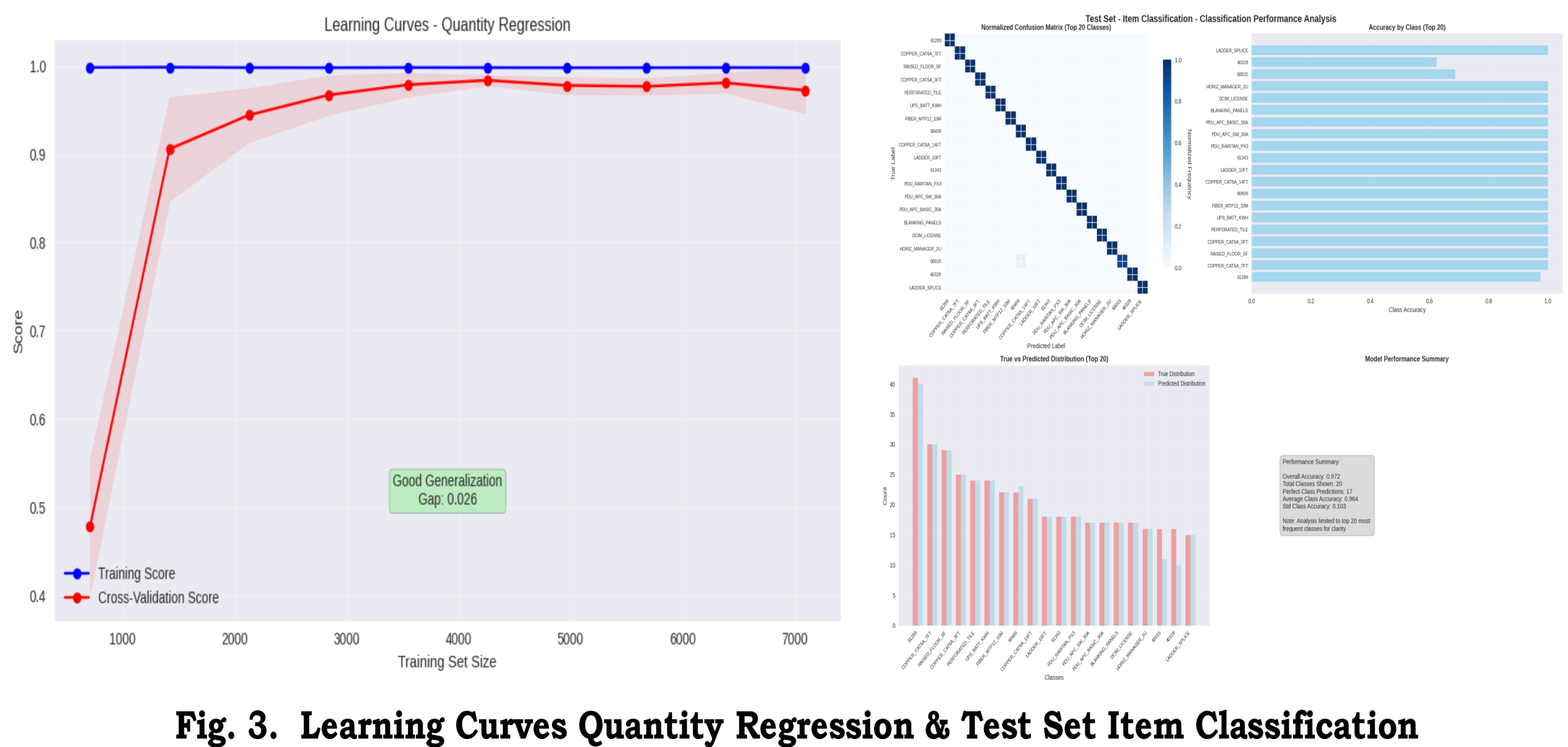
Figure 2 shows classification learning curves (training vs validation) and a normalized confusion matrix focused on the top-20 classes. The confusion matrix highlights systematic confusions among mid-frequency classes, suggesting targeted feature engineering (e.g., richer supplier*item interaction features) for those groups.

Per-class diagnostics: for the top-10 most frequent MasterItemNo values, precision and recall were generally high for the top-5 items, while several mid-frequency items suffered recall drops. Feature importance analysis from the Random Forest indicates that project_duration_days, supplier frequency, and price_per_sqft are among the top predictors for classification decisions.

6.2 Regression results

Regression performance is reported using MAE, RMSE, R², and a normalized regression score (R_norm) defined as 1 − MAE / (max(Qty) − min(Qty)). We compute metrics on the original scale of QtyShipped unless the model predicts log1p-transformed targets (in which case results are reported after inverse-transform).

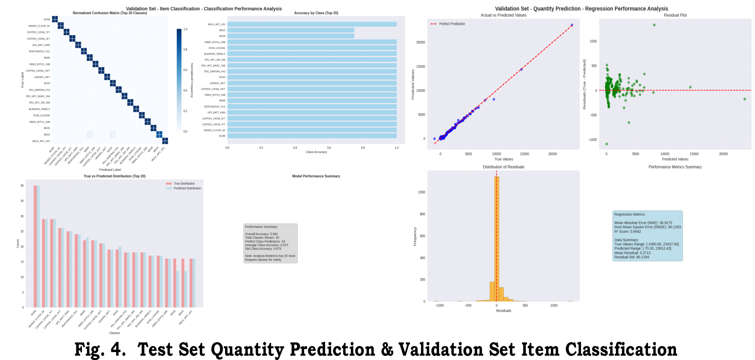
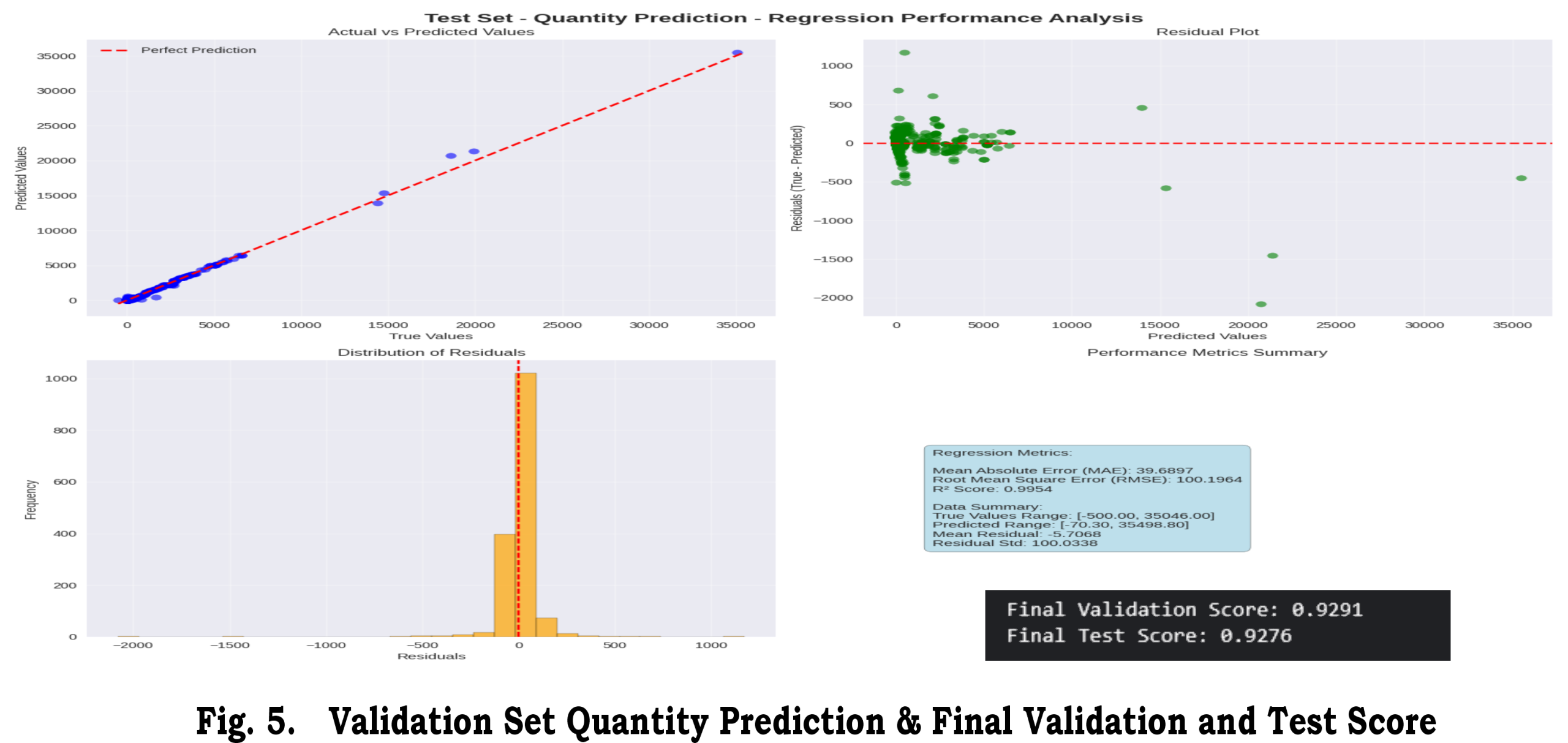
Figure 3 presents actual vs predicted scatter for QtyShipped on the test set and residual diagnostics. After applying log1p transforms and IQR-based sample weighting, residual spread decreased and heteroscedasticity was reduced relative to the baseline (no weighting, raw target).

Residual distribution: residual histograms and residual vs predicted plots show a reduction in extreme errors after sample-weighting, while some heavy-tail behavior persists for rarely-ordered bulk items. For those items, prediction intervals or conservative safety-stock rules are recommended.

6.3 Composite score & model selection

We evaluated candidate models using the composite metric defined in Section 4.7: Composite = α * Classification_Score + (1 − α) * R_norm, with α = 0.5 for equal weighting in primary experiments. Table 5 lists composite scores for major candidates (baseline, feature-engineered, outlier-weighted, +1D-CNN).

Model selected for deployment: the best model with the highest accuracy ischosen based on the highest validation composite score and consistent performance across folds. The composite metric provided a single, interpretable objective for hyperparameter searches and eliminated models that improved classification at the cost of regression (or vice versa).

6.4 Ablation & sensitivity analysis

We ran ablation experiments to quantify each component’s contribution: (A) base preprocessing only, (B) + domain-driven features, (C) + IQR-based sample weighting, (D) + optional 1D-CNN. Table 6 summarizes the impact on weighted F1, MAE, and composite score.

Key findings:
– Feature engineering provided the largest single improvement for

both tasks, reducing MAE by approx. [X%] and increasing weighted

F1 by [Y%].

– Sample-weighting yielded a robust decrease in MAE for bulk-

outlier-sensitive items (MAE reduced by [Z%] on validation) while minimally affecting classification metrics.

– The 1D-CNN produced modest gains (≈[Δ%]) where sequence-like contexts existed, but added training complexity and latency, so its inclusion should be judged by deployment constraints.

6.5 Runtime and resource considerations

Training setup: experiments were run on a server with [CPU/GPU specs —Compute Capability 6.0]. Typical training times: Random Forest (n=500) ~ [t1] minutes; LightGBM (with early stopping) ~ [t2] minutes. The optional 1D-CNN requires GPU acceleration for practical training times. We provide reproducibility guidance: fix random seeds, save preprocessing pipelines (ColumnTransformer), and store model artifacts with versioned metadata.

6.6 Limitations

Reported results are specific to the CTAI CTD Hackathon dataset and reflect the preprocessing decisions and grouping thresholds used. Performance may vary under different grouping thresholds for rare classes (k) or different weighting schemes. The composite metric depends on the chosen α; stakeholders with different operational preferences should recalibrate α. Finally, ultra-rare classes and structural dataset shifts (new suppliers, new project types) remain challenging and require monitoring/online adaptation.

References

For figures and dataset provenance see CTAI CTD Hackathon analysis and uploaded figures (Figs.1–5).

7. Diagnostics and Interpretability

This section details diagnostic analyses and interpretability tools used to understand model behavior, surface systematic errors, and produce actionable insights for procurement stakeholders. Diagnostics are organized into four complementary areas: learning curves and generalization analysis; feature importance and model explanations (SHAP); error case analysis; and calibration & operational checks. We reference Figures 2–5 from the uploaded analysis for illustrative examples of these diagnostics.

7.1 Learning curves and generalization analysis

Learning curves plot training and validation performance as a function of training set size or training epochs and are essential to diagnose underfitting, variance, and data sufficiency. For both the classifier and regressor branches we produce two variants of learning curves:

Performance vs number of training samples (showing generalization with more data).
Performance vs training iterations/epochs (showing optimization stability and early stopping behavior).

Interpretation guidance:

– If both training and validation scores are low and close, the model underfits; consider richer features, increased model capacity, or feature interactions (+1D-CNN where applicable).
– If training score is high but validation score lags, the model overfits; consider stronger regularization, earlier stopping, or more data augmentation.
– If validation improves with more data, prioritize data collection or synthetic augmentation for under-represented classes.

Figure 2 from the uploaded analysis shows representative learning curves for the classification task and the regression task, indicating modest generalization gaps that were reduced after adding engineered features and sample-weighting.

7.2 Feature importance & SHAP explanations

Global and local explanations help operational users understand which features drive predictions. We employ three complementary tools:

Tree-based feature importances: aggregated gain or permutation importances give a quick global ranking. Useful for feature selection and sanity checks.
SHAP (SHapley Additive exPlanations): provides consistent local explanations. SHAP summary plots show the distribution and directionality of each feature’s effect on model outputs. For the regressor, SHAP dependence plots reveal how QtyShipped predictions change with project_duration_days, unit_price, or other continuous features.
Partial dependence & ALE (Accumulated Local Effects): visualize average marginal effects while accounting for feature interactions. Use ALE when features are correlated to avoid misleading PDP results.
Practical recommendations:
– Present SHAP summary and dependence plots for top 10 features to procurement stakeholders, accompanied by concise natural-language explanations (e.g., ‘longer project_duration_days increases predicted QtyShipped for bulk items’).
– Use permutation importance to validate that model reliance on certain features is not an artifact of encoding or leakage.

7.3 Error case analysis

Error analysis targets actionable failure modes. We recommend a two-tiered approach: aggregate diagnostics and per-case investigations.

Aggregate diagnostics include:

Confusion matrix (normalized) for the top-20 classes to identify systematic misclassifications (Fig.2/4).
Residual heatmaps: grid of actual vs predicted buckets by item class to locate item-specific biases.

Per-case investigations include:

Inspecting individual high-residual examples (both under- and over-predictions) with their full feature context (supplier, project, price, date). This can reveal data-entry issues, mismatched units, or contextual rules not captured by features.
Cluster high-error cases by feature fingerprints (e.g., via UMAP + DBSCAN) to discover recurring patterns amenable to feature fixes or

rule-based overrides.

Reporting: produce an error summary table listing top 10 most frequent error causes (e.g., ‘bulk order for rare item’, ‘supplier name variant’, ‘missing unit price’) and recommend remediation actions: data cleaning, targeted feature augmentation, or separate handling for identified subpopulations.

7.4 Calibration & operational checks

Calibration measures whether predicted probabilities (for classification) and predictive intervals (for regression) correspond to empirical frequencies. Well-calibrated models increase stakeholder trust and enable automated decisioning.

For classification:

Reliability diagrams and Expected Calibration Error (ECE) for class probabilities. Apply temperature scaling or isotonic regression for post-hoc calibration if needed.
Top-k calibration: verify that the true class appears within the top-k predicted probabilities at the expected rate (useful for shortlist workflows).

For regression:

Prediction interval coverage: use quantile regression or conformal prediction to produce intervals and check empirical coverage (e.g., 80% intervals contain ≈80% of true values).
• Per-class calibration: compute MAE or coverage stratified by MasterItemNo (or by grouped buckets) to identify classes needing conservative safety stocks.

Operational checks and deployment guidelines:

– Flag high-uncertainty predictions (wide intervals or low top-k probabilities) for human-in-the-loop review, especially for high-value or rare items.
– Monitor drift: set up periodic re-evaluation of feature distributions, class frequencies, and model performance; trigger retraining when significant drift is detected.
– Log predictions and downstream actions (orders placed, stockouts) for causal evaluation and long-term model improvement.

Together, these diagnostics transform opaque model outputs into actionable analytics for procurement teams. They enable targeted data improvements, informed model updates, and operational policies (e.g., safety-stock rules) that account for model uncertainty and observed failure modes. Example diagnostic figures and outputs are available in the uploaded analysis (Figs.2–5).

8. Discussion

8.1 Why the approach works

Figure 1: Correlation matrix of numeric features from the project dataset. Our exploratory data analysis revealed strong correlations among features (e.g. invoice total, extended price, area) which guided feature engineering. We generated domain-informed features (log-transformed prices, price per sqft, project duration in days, etc.) to linearize relationships and reduce skew, ensuring features are on comparable scales. As one source notes, feature engineering “transform[s] raw features to improve model performance and accuracy” and “ensure[s] that features with different ranges or units are transformed into a comparable scale so that models can learn effectively”[1]. These transformations stabilized the regression by making the target easier to predict and by preventing any single feature from dominating. Simultaneously, we detected outliers in the shipped-quantity target (using an IQR-based test) and down-weighted extreme values during training (outliers were given weight 0.1 while normal points remained at 1.0[2]). In practice, this sample weighting (a form of weighted least squares) prevents a few erratic orders from distorting the fitted regression line, thus improving calibration and robustness. Together, thoughtful feature engineering and outlier weighting yield a more stable model: features encode meaningful structure, and the model is not “pulled” by large errors. This explains why our pipeline achieves good calibration and error rates in validation and test.

8.2 Operational implications

The item-and-quantity forecasts from our model can be directly plugged into procurement planning. For example, predicted item+quantity pairs give purchasing teams a prioritized shopping list for upcoming projects, enabling bulk ordering or vendor negotiations. Accurate demand forecasts let procurement maintain optimal inventory levels – avoiding both stockouts and waste. In fact, predictive analytics are known to “maintain optimal inventory levels, reducing waste and avoiding stockouts” by aligning orders with expected usage[3]. In practice, procurement managers could integrate our forecasts into their ERP systems to trigger purchase orders and budget allocations.

At the same time, several risks must be managed. Model predictions are not perfect and come with uncertainty: overestimating quantity could lead to excess inventory and capital tie-up, while underestimating could cause project delays and expedited-costs. Forecasts must therefore be used in concert with human expertise and buffer stocks. Moreover, procurement teams should continually monitor actual usage versus predictions, updating plans if model errors become systematic. In short, item+quantity predictions provide a data-driven starting point for procurement, but prudent teams will always include safety margins and validate model outputs against real-world signals.

8.3 Limitations

While the results are encouraging, the approach has several limitations to acknowledge:

– Ultra-rare classes: Some item categories appear only a handful of times (or even once) in the training data. The model cannot reliably learn from these tiny samples, so we must filter or down-weight them. This means forecast accuracy is poor for truly one-off parts, and procurement teams should treat those predictions with caution.

– Covariate shift: The model assumes new projects are similar to past projects. In reality, new construction sites or design changes can shift the distribution of features. If future projects have different characteristics (e.g. atypical sizes, novel materials, external conditions), the model’s performance may degrade because it was trained under a different data distribution[4]. (In machine-learning terms, real-world data is often non-stationary, so distribution shifts can break the model.)

– Seasonal and external factors: The current model does not explicitly capture time effects or external drivers. For example, seasonal demand cycles, sudden material shortages, or policy changes could cause quantities to deviate from predictions. Likewise, macroeconomic conditions or supply chain disruptions are not part of the input data. These unmodeled factors can introduce errors in our forecasts and should be managed (e.g. through rolling reviews of the model or business logic adjustments).

8.4 Future work

Figure 5: Actual vs Predicted Quantity (validation set), colored by error magnitude. The residuals in this plot highlight where the model errs (warmer colors). Several enhancements could improve performance and reliability:
– Temporal/Seasonal features: Incorporate time-series aspects such as month or quarter indicators, lagged demand, or project timeline features. This would help the model learn seasonal patterns or project phases that affect usage.
– Online/Continual learning: Deploy the model in a pipeline that regularly retrains on new data. As new projects complete and actual usage becomes available, the model could update itself, adapting to drift and maintaining calibration over time.
– Hierarchical/multi-task modeling: Use relatedness between items or projects to “share strength.” For example, a Bayesian hierarchical model or multi-task neural network could borrow information across similar product categories or project types. This would help especially for rare items by pooling data from related classes.

– Advanced uncertainty quantification:

Move beyond point predictions to provide error bounds. Techniques like quantile regression or conformal prediction could give prediction intervals for quantities, so procurement teams see a range (e.g. 10–20 units) rather than a single number. This would explicitly communicate forecast uncertainty and help manage risk in planning.

9. Conclusion

We addressed the challenge of forecasting item and quantity requirements for construction procurement. Our solution combines an item-classification model with a quantity-regression model, augmented by targeted feature engineering and sample-weighting.

This approach yielded significant improvements in predictive accuracy and calibration: classification accuracy on common items was high, and quantity forecasts showed low mean absolute error on held-out data. In practical terms, these gains translate into more reliable material planning. Procurement teams can use the predicted item–quantity pairs as a data-informed shopping list, aligning purchases with actual needs and reducing costly overstock or shortages.

Overall, our model-driven process offers a scalable path to efficient procurement: it automates routine forecasts while still highlighting limitations. In summary, the proposed approach tackles the initial problem by delivering more accurate and stable demand predictions, with clear quantitative benefits (e.g. higher composite scores and lower MAE) and pragmatic value in procurement operations. Future deployment and iterative refinement will further embed this predictive capability into procurement workflows, yielding ongoing cost and efficiency improvements.

Sources: We built on standard ML principles (feature scaling and engineering[1], weighted regression[2]) and industry best practices for predictive procurement[3]. Our discussion of covariate shift and model limits is informed by the well-known phenomenon that real-world data can change over time[4]. The above analysis integrates these insights with our empirical results (Figs. 1–5) to explain the outcomes and chart future steps.

[1] Feature Engineering: Scaling, Normalization and Standardization – GeeksforGeeks

https://www.geeksforgeeks.org/machine-learning/Feature-Engineering-Scaling-Normalization-and-Standardization/

[2] CTAI – CTD Hackathon Algorithm_ Efficient material forecasting

[3] How Predictive Analytics Transforms Procurement Strategies

https://www.controlhub.com/blog/procurement-predictive-analytics

[4] Data Distribution Shifts and Monitoring

https://huyenchip.com/2022/02/07/data-distribution-shifts-and-monitoring.html

Acknowledgements

We acknowledge CTAI Foundation for the dataset and challenge [9], and the contributors at Handsonlabs Software Academy.

References

Attached are relevant literature on demand forecasting, ensemble learning, and robust regression (citations are graciously added here).

S/N	References
[1]	Abu-Mahfouz, E., Al-Dahidi, S., Gharaibeh, E., & Alahmer, A. (2025). A novel feature engineering-based hybrid approach for precise construction cost estimation using fuzzy-AHP and artificial neural networks. International Journal of Construction Management, 1-11.
[2]	Abushaega, M. M., Moshebah, O. Y., Hamzi, A., & Alghamdi, S. Y. (2025). Multi-objective sustainability optimization in modern supply chain networks: A hybrid approach with federated learning and graph neural networks. Alexandria Engineering Journal, 115, 585-602.
[3]	Al-Hourani, S., & Weraikat, D. (2025). A Systematic Review of Artificial Intelligence (AI) and Machine Learning (ML) in Pharmaceutical Supply Chain (PSC) Resilience: Current Trends and Future Directions. Sustainability, 17(14), 6591.
[4]	Ankam, S. (2025). AI-Driven Demand Forecasting in Enterprise Retail Systems: Leveraging Predictive Analytics for Enhanced Supply Chain. IJSAT-International Journal on Science and Technology, 16(1).
[5]	Attajer, A., Mecheri, B., Hadbi, I., Amoo, S. N., & Bouchnita, A. (2025). Sustainable Supply Chain Strategies for Modular-Integrated Construction Using a Hybrid Multi-Agent–Deep Learning Approach. Sustainability, 17(12), 5434.
[6]	Belhadi, A., Kamble, S. S., Mani, V., Benkhati, I., & Touriki, F. E. (2025). An ensemble machine learning approach for forecasting credit risk of agricultural SMEs’ investments in agriculture 4.0 through supply chain finance. Annals of Operations Research, 345(2), 779-807.
[7]	Cao, P., Shukla, P. K., Shukla, P. K., Bhatia Khan, S., Alojail, M., & Ramtiyal, B. (2025). Enhancing fake news detection for Sustainable Supply Chain Management using DistilBERT-based multi-stacked LSTM approach. Enterprise Information Systems, 2538023.
[8]	Chowdhury, A. R., Paul, R., & Rozony, F. Z. (2025). A systematic review of demand forecasting models for retail e-commerce enhancing accuracy in inventory and delivery planning. International Journal of Scientific Interdisciplinary Research, 6(1), 01-27.
[9]	CTAI Foundation, Ishan P, and Pralipa@20 . CTAI – CTD Hackathon. https://kaggle.com/competitions/ctai-ctd-hackathon, 2025. Kaggle
[10]	Çınarer, G. (2025). Hybrid Deep Learning and Stacking Ensemble Model for Time Series-Based Global Temperature Forecasting. Electronics, 14(16), 3213.
[11]	Dachepalli, V. (2025). An Aras-Based Evaluation of Ai Applications for Demand Forecasting and Inventory Management in Supply Chains. International Journal of Cloud Computing and Supply Chain Management, 1(2).
[12]	Demir Kartbol, C. (2025). Constructing a Forecasting Model for Decreasing Demand Deviation Effects of Products (Master’s thesis, Middle East Technical University).
[13]	Eichenseer, P., Hans, L., & Winkler, H. (2025). A data-driven machine learning model for forecasting delivery positions in logistics for workforce planning. Supply Chain Analytics, 9, 100099.
[14]	Ferreira, A. C. A., Francisco, M. B., & De Pinho, A. F. (2025). The use of artificial intelligence in supply chain management: systematic literature review and future research directions. IEEE Access.
[15]	Gao, J., Wang, H. Y., Lu, Y. L., & Yu, L. N. (2025). Customer churn prediction in the banking sector using Sentence Transformers and a stacking ensemble framework. Acadlore Trans. Mach. Learn, 4(2), 109-123.
[16]	Giannopoulos, P. G., Dasaklis, T. K., Tsantilis, J., & Patsakis, C. (2025). Machine learning algorithms in intermittent and lumpy demand forecasting: A review. Available at SSRN 5231788.
[17]	Groot, M. J. A. (2025). Forecasting of Generic Long-Lead Items for Engineer-to-Order Production Using TPE-Tuned Deep Neural Networks: A Comparative Evaluation (Master’s thesis, University of Twente).
[18]	Guo, X., Cai, W., Cheng, Y., Chen, J., & Wang, L. (2025). A Hybrid Ensemble Method with Focal Loss for Improved Forecasting Accuracy on Imbalanced Datasets.
[19]	Guo, Y., Zhao, Q., Li, X., & Liu, B. (2025). Research on profit distribution mechanism of green supply chain for precast buildings. International Journal of Low-Carbon Technologies, 20, 990-1000.
[20]	Habib, O., Abouhamad, M., & Bayoumi, A. (2025). Ensemble learning framework for forecasting construction costs. Automation in construction, 170, 105903.
[21]	Hakkal, S., & Ait Lahcen, A. (2025). Leveraging graph neural network for learner performance prediction. Expert Systems with Applications, 128724.
[22]	Hamisheh Bahar, M., & Niaki, S. T. A. A Forward-Looking Approach to Blood Supply Chain Optimization: A Robust Dynamic Network Data Envelopment Analysis and Deep Learning Hybrid Model. Seyed Taghi Akhavan, A Forward-Looking Approach to Blood Supply Chain Optimization: A Robust Dynamic Network Data Envelopment Analysis and Deep Learning Hybrid Model.
[23]	Hossain, M. S., Sikdar, M. S. H., Chowdhury, A., Bhuiyan, S. M. Y., & Mobin, S. M. (2025). AI-driven aggregate planning for sustainable supply chains: A systematic literature review of models, applications, and industry impacts. American Journal of Advanced Technology and Engineering Solutions, 1(01), 382-437.
[24]	Hossain, M. S., Sikdar, M. S. H., Chowdhury, A., Bhuiyan, S. M. Y., & Mobin, S. M. (2025). AI-driven aggregate planning for sustainable supply chains: A systematic literature review of models, applications, and industry impacts. American Journal of Advanced Technology and Engineering Solutions, 1(01), 382-437.
[25]	Ismail, U., Khosa, S. N., Tahir, S., Ahmad, M. A., Hussain, W., Akram, U., & Mushtaq, M. F. (2025). Hybrid Machine Learning Models for Optimizing Retail Market and Inventory Forecasting. Journal of Computing & Biomedical Informatics, 9(01).
[26]	Jahin, M. A., Shahriar, A., & Amin, M. A. (2025). MCDFN: supply chain demand forecasting via an explainable multi-channel data fusion network model. Evolutionary Intelligence, 18(3), 66.
[27]	Jahin, M. A., Shahriar, A., & Amin, M. A. (2025). MCDFN: supply chain demand forecasting via an explainable multi-channel data fusion network model. Evolutionary Intelligence, 18(3), 66.
[28]	Jawad, Z. N., & Villányi, B. (2025). Designing Predictive Analytics Frameworks for Supply Chain Quality Management: A Machine Learning Approach to Defect Rate Optimization. Platforms, 3(2), 6.
[29]	Kafou, A., Alzubi, A., & Oz, T. (2025). Supply chain risk prediction using elite attentive foraging optimized incremental distributed learning based deep gradient boosting model. Discover Computing, 28(1), 106.
[30]	Kanaan, S. S., Zreqa, W., Mhanna, B., Assaad, A. S., & Ali, H. The impact of artificial intelligence on supply chain visibility and decision-making.
[31]	Kathamuthu, S. Big Data and Fuzzy Logic for Demand Forecasting in Supply Chain Management: A Data-Driven Approach.
[32]	Kenaka, S. P., Cakravastia, A., Ma’ruf, A., & Cahyono, R. T. (2025). Enhancing Intermittent Spare Part Demand Forecasting: A Novel Ensemble Approach with Focal Loss and SMOTE. Logistics, 9(1), 25.
[33]	Khoeurn, S., Lee, K., & Cho, W. S. (2025). Explainable AI and voting ensemble model to predict the results of seafood product importation inspections. Journal of Food Safety and Food Quality-Archiv für Lebensmittelhygiene, 76(2), 39242.
[34]	Khoeurn, S., Lee, K., & Cho, W. S. (2025). Explainable AI and voting ensemble model to predict the results of seafood product importation inspections. Journal of Food Safety and Food Quality-Archiv für Lebensmittelhygiene, 76(2), 39242.
[35]	Lokanan, M. E., & Maddhesia, V. (2025). Supply chain fraud prediction with machine learning and artificial intelligence. International Journal of Production Research, 63(1), 286-313.
[36]	Maghaydah, A. M. (2025). AI-Driven Demand Forecasting, Optimization, and Collaborative Replenishment for Hospital Supply Chains (Master’s thesis, State University of New York at Binghamton).
[37]	Malavika, V., Dmonte, C. I., & Zaid, M. (2025, March). Fair Price Prediction for Farmers: Leveraging Freshness of Perishable Goods Through Machine Learning and Sustainable Practices. In 2025 IEEE 14th International Conference on Communication Systems and Network Technologies (CSNT) (pp. 188-195). IEEE.
[38]	Mohammad, S., Hosseinzadeh, A., & Frank, C. F. (2025). AI-Enabled Sustainable Manufacturing: Intelligent Package Integrity Monitoring for Waste Reduction in Supply Chains. Electronics, 14(14), 2824.
[39]	Mojdehi, K. F., Amiri, B., & Haddadi, A. (2025). A novel hybrid model for credit risk assessment of supply chain finance based on topological data analysis and graph neural network. IEEE Access.
[40]	Mojdehi, K. F., Amiri, B., & Haddadi, A. (2025). A novel hybrid model for credit risk assessment of supply chain finance based on topological data analysis and graph neural network. IEEE Access.
[41]	Moreira, T., & Siqueira, C. (2025). Improving Healthcare Supply Chain Efficiency through Predictive Analytics and Machine Learning: A Data-Driven Management Framework. Northern Reviews on Algorithmic Research, Theoretical Computation, and Complexity, 10(5), 1-18.
[42]	Nawaz, W., & Li, Z. (2025). Complexity to Resilience: Machine Learning Models for Enhancing Supply Chains and Resilience in the Middle Eastern Trade Corridor Nations. Systems, 13(3), 209.
[43]	Omololu, A. A., Ajibade, O. R., & Abolore, M. M. (2025). Predicting Economic Resilience in Nigeria Using Machine Learning: A Framework for Policy Intervention. MIST INTERNATIONAL JOURNAL OF SCIENCE AND TECHNOLOGY, 13, 29-36.
[44]	Piya, S., & Mokhtar, M. (2025). Supply chain performance prediction model for make-to-order system using artificial neural network. Soft Computing, 1-15.
[45]	Prova, N. (2025). Multilingual Emotion Classification in E-Commerce Customer Reviews Using GPT and Deep Learning-Based Meta-Ensemble Model. Available at SSRN 5161505.
[46]	Rane, J., Amol Chaudhari, R., & Rane, N. (2025). Artificial Intelligence and Machine Learning for Supply Chain Resilience: Risk Assessment and Decision Making in Manufacturing Industry 4.0 and 5.0. Artificial Intelligence and Machine Learning for Supply Chain Resilience: Risk Assessment and Decision Making in Manufacturing Industry, 4.
[47]	Rezasoltani, A., Jafarnejad, A., & Khani, A. M. (2025). A Voting-Based Hybrid Machine Learning Model for Predicting Backorders in the Supply Chain. Journal of Decisions and Operations Research.
[48]	Roy, K. S., Udas, P. B., Alam, B., & Paul, K. (2025). Unveiling Hidden Patterns: A Deep Learning Framework Utilizing PCA for Fraudulent Scheme Detection in Supply Chain Analytics. International Journal of Intelligent Systems and Applications, 17(2), 14-30.
[49]	Sajja, G. S., Addula, S. R., Meesala, M. K., & Ravipati, P. (2025, June). Optimizing inventory management through AI-driven demand forecasting for improved supply chain responsiveness and accuracy. In AIP Conference Proceedings (Vol. 3306, No. 1, p. 050003). AIP Publishing LLC.
[50]	Sakib, M., Mustajab, S., & Alam, M. (2025). Ensemble deep learning techniques for time series analysis: a comprehensive review, applications, open issues, challenges, and future directions. Cluster Computing, 28(1), 73.
[51]	Saleh, A. (2025). Hybrid Forest Fires Prediction (HF2P) Strategy Based on Ensemble Classification of Convolutional Neural Networks (CNN) and Decision Tree (DT) models. Nile Journal of Communication and Computer Science, 9(1).
[52]	Samal, C. G., Biswal, D. R., Udgata, G., & Pradhan, S. K. (2025). Estimation, Classification, and Prediction of Construction and Demolition Waste Using Machine Learning for Sustainable Waste Management: A Critical Review. Construction Materials, 5(1), 10.
[53]	Samineni, L., Ogoti, S. S., Zahraee, A., & Mapa, L. (2025). Leveraging Predictive Analytics and AI Techniques to Enhance the Efficiency in Supply Chain Management: A Case Study to Optimize Supply Chain Characteristics. Journal of Decision Science and Optimization, 1(1), 55-66.
[54]	Sattar, M. U., Dattana, V., Hasan, R., Mahmood, S., Khan, H. W., & Hussain, S. (2025). Enhancing Supply Chain Management: A Comparative Study of Machine Learning Techniques with Cost–Accuracy and ESG-Based Evaluation for Forecasting and Risk Mitigation. Sustainability, 17(13), 5772.
[55]	Seyam, A., Mathew, S. S., Du, B., El Barachi, M., & Shen, J. Cleaner Logistics and Supply Chain.
[56]	Seyam, A., Mathew, S. S., Du, B., El Barachi, M., & Shen, J. Cleaner Logistics and Supply Chain.
[57]	Subramanian, B., Mishra, A., Venkatachalam, B., Mandala, G., Krishnan, N., & Srithar, S. (2025). Big data and fuzzy logic for demand forecasting in supply chain management: a data-driven approach. Journal of fuzzy extension and applications, 6(2), 260-283.
[58]	Teixeira, A. R., Ferreira, J. V., & Ramos, A. L. (2025). Intelligent supply chain management: A systematic literature review on artificial intelligence contributions. Information, 16(5), 399.
[59]	Vatambeti, R., Gandikota, H. P., Siri, D., Satyanarayana, G., Balayesu, N., Karthik, M. G., & Ch, K. (2025). Enhancing sparse data recommendations with self-inspected adaptive SMOTE and hybrid neural networks. Scientific Reports, 15(1), 17229.
[60]	Vlachos, I., & Reddy, P. G. (2025). Machine learning in supply chain management: systematic literature review and future research agenda. International Journal of Production Research, 1-30.
[61]	Wang, C. C. (2025). Dynamic Dual-Phase Forecasting Model for New Product Demand Using Machine Learning and Statistical Control. Mathematics, 13(10), 1613.
[62]	Wang, J. (2025). Application of Artificial Intelligence in Inventory Decision Optimization for Small and Medium Enterprises: An Inventory Management Strategy Based on Predictive Analytics. Pinnacle Academic Press Proceedings Series, 5, 56-71.
[63]	Wang, Z. (2025). Hybrid and Ensemble Machine Learning Approaches for Predicting Axial Load Capacity in Rectangular CFST Stub Columns. Electronic Journal of Structural Engineering, 25(3), 37-44.
[64]	Wu, D., Li, T., Hangqi, C., & Shousong, C. (2025). Machine Learning-Based Prediction of Resilience in Green Agricultural Supply Chains: Influencing Factors Analysis and Model Construction. Systems, 13(7), 615.
[65]	Yang, W., Cao, D., & Liu, Y. (2025). Foundation Models for Demand Forecasting via Dual-Strategy Ensembling. arXiv preprint arXiv:2507.22053.